Modeling stomatal conductance (gs) is a key challenge in vegetation models and land surface models, and various approaches have been developed including statistics- and optimality-based models. The stomatal model is typically used along with the canopy radiative model, which provides the former with necessary inputs like photosynthetically active radiation (PAR) and temperature (T) to compute photosynthesis and then gs. In model world practice, gs is typically computed at a steady state, meaning that model parameters (such as photosynthetic rate [A], transpiration rate (E), gs, PAR, and T) agree numerically. This assumption is fine for most models as their canopy models are simple enough and the computation resource required to derive the steady state is low.
However, finding a similar steady state for complicated canopy models as in CliMA Land is overwhelming. For example, any change in gs would lead to changes in A and E, and thus leaf latend heat flux, leaf temperature, longwave radiation, hydraulic profiles, etc.
Moreover, the steady-state assumption could break the mass and energy conservation. If leaf water content and heat capacity are considered, but the final water and heat flux are all at steady state, then how do we account for the changes in water mass and total energy?
Most importantly, the soil-plant-air continuum in nature will NEVER be at a steady state, say the sun is moving all the time, wind is randomly changing leaf positions, soil water contents are changing, and plant physiology is responding. For all these reasons, we’d better model the land surface processes prognostically.
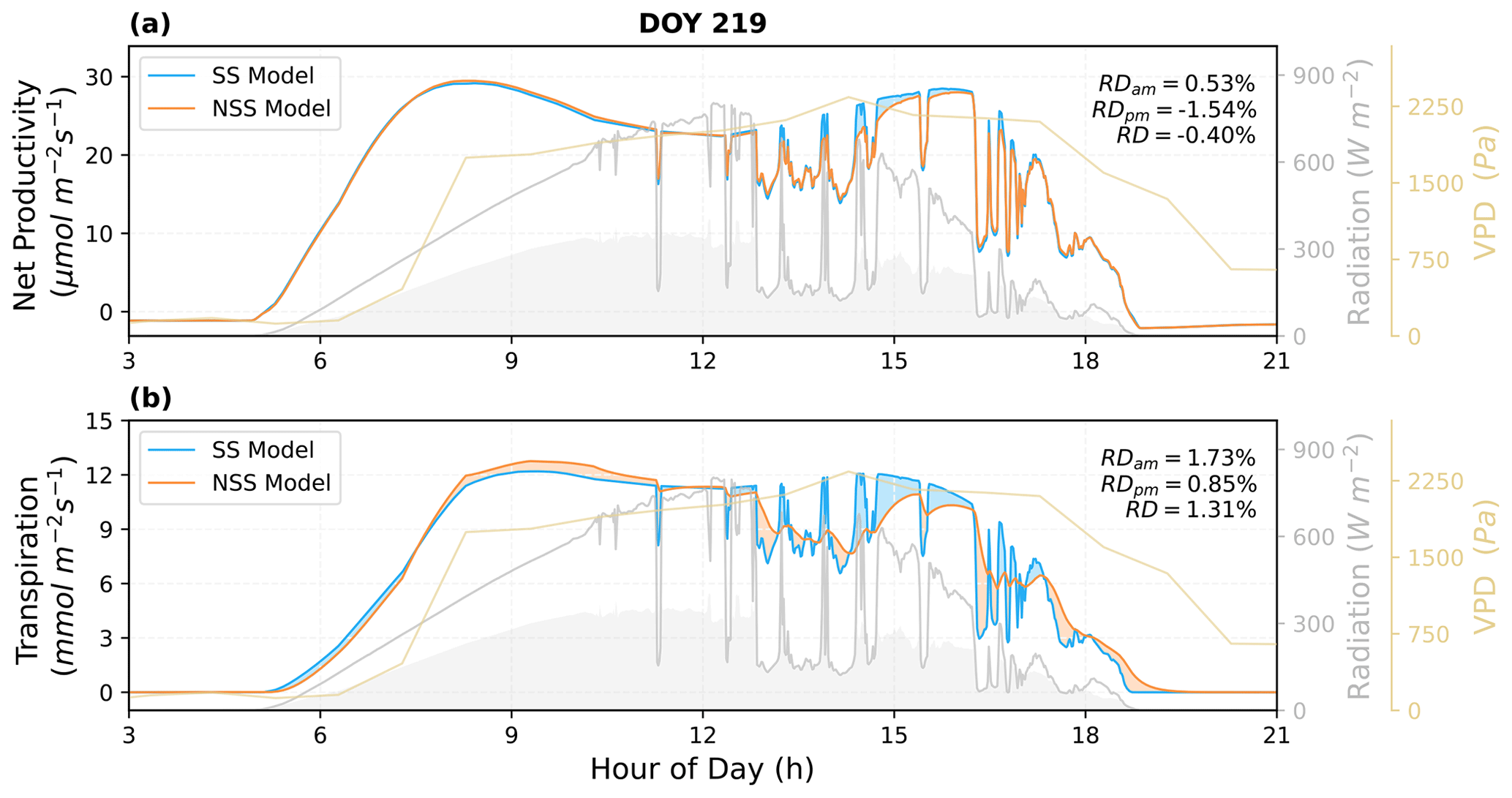
In the recent research led by Ke Liu (Liu et al., 2024; Biogeosciences), we evaluated the impacts of modeling gs at non-steady state using CliMA Land. We found that, as stomata open “slowly” (compared to immediately at steady state), gs would be lower than steady state models in the morning time in an ideal environment without cloud. Comparatively, as stomata close “slowly”, gs would be higher than the steady-state assumption in the afternoon in the ideal environment. In this case, these differences could cancel out, but it still suggested that modelers had messed up the timing. Notably, the natural environment is never ideal following a sine or cosine function, and plants are experiencing random fluctuations in radiation, dry air, etc. These resulted in elevated differences between steady-state and non-steady-state modeling (Fig. 1).

There are many benefits for models to take the non-steady state approach, particularly that it is more realistic! There are also more implications from the study, please check out the paper for more details. Yet, there are still a lot of problems to resolve in the future, such as
- How to best represent the prognostic gs (other formulations)?
- Do plants have different time constants when opening and closing the stomata?
- Do sunlit and shaded leaves have different time constants?
I am keen to see follow-up studies that address these problems. Together, we can make the vegetation and land surface models more realistic.